376,031 views | 01:35:29
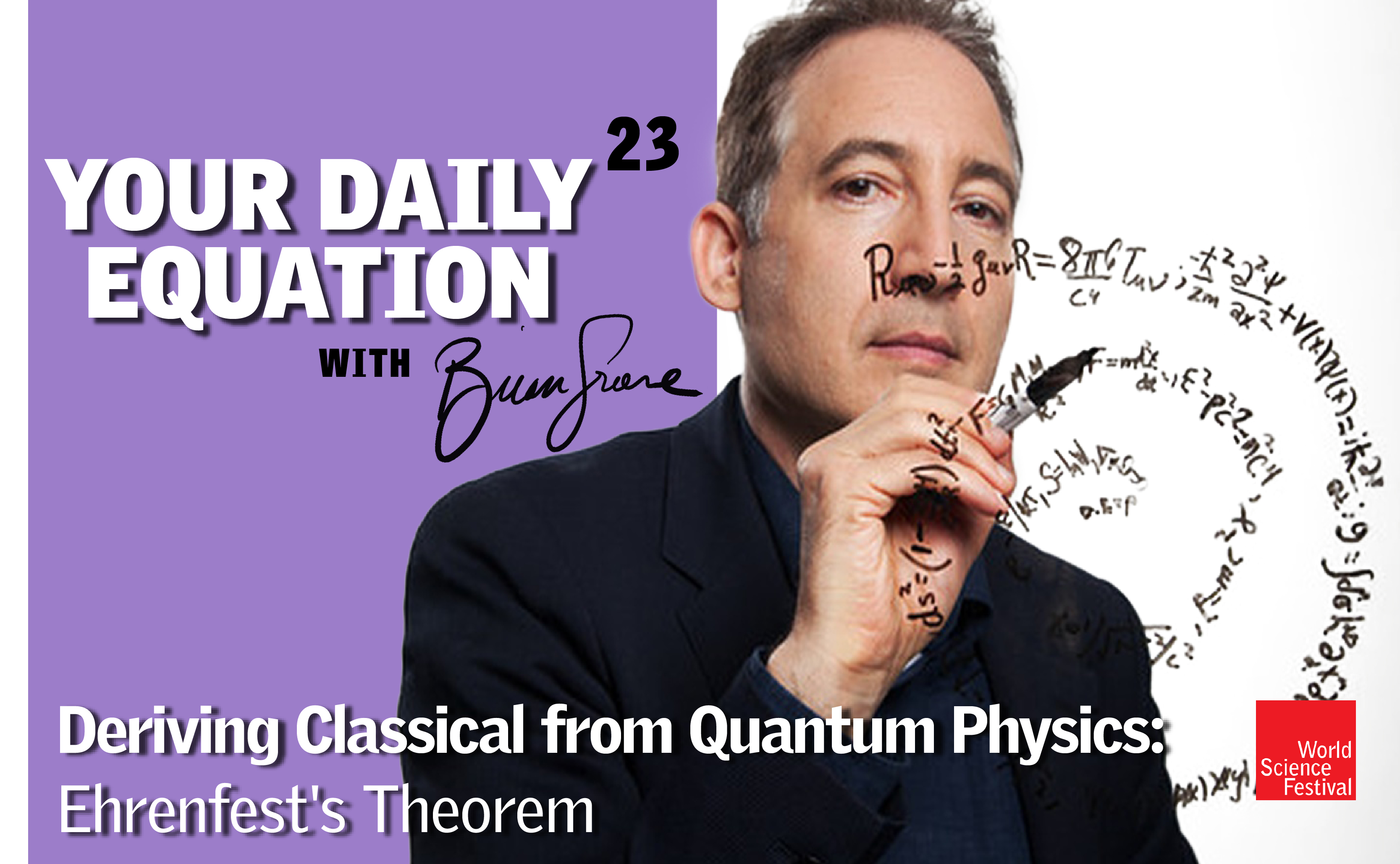
Join us for #YourDailyEquation with Brian Greene. Every Mon - Fri at 3pm EDT, Brian Greene will offer brief and breezy discussions of pivotal equations. Even if your math is a bit rusty, tune in for accessible and exciting stories of nature and numbers that will allow you to see the universe in a new way. Classical and Quantum Physics describe reality in completely different ways. Yet, in 1927, Paul Ehrenfest showed how Newton's equation could be derived from Schrödinger's, establishing a deep continuity in our understanding of the physical universe. Join Brian Greene for a brief explanation of Ehrenfest's essential idea as well as the mathematical manipulations he required to realize it.Learn More
Speaker 1:
Hey everyone, welcome back to Your Daily Equation. And today I’m going to address a question that I’m kind of asked all the time in one form or another which basically asks, for instance when do you have to make use of special relativity? At what speed do you need to use the equations of special relativity? Or when do you really need to use general relativity? What mass scale do the equations of general relativity kick in or at what lane scale? How small do you have to go before you need to use the laws of quantum mechanics?
And of course I understand the intuition behind the question completely. When we learn about physics, we first learned about classical mechanics and Newton’s laws, and then we learn about these more refined descriptions of the world, quantum mechanics, special relativity, general relativity and so forth. So you naturally wonder, “Okay, when do I need to use those theories?” Now the fact of the matter is, in principle you really need to use those theories all the time in the sense that those theories, they apply everywhere at all mass scales, at all speeds, at all lane scales. The more refined description that we have achieved through our monomer search is the right description.
But of course, if you’re plotting the course of a rocket going to the moon, nobody uses quantum mechanics. You could use quantum mechanics, at least in principle, but Newton’s laws of motion from classical mechanics are such a good approximation that those are the equations that we use. They’re a much simpler description of a rocket going to the moon and they’re so fantastically accurate that we don’t need to use a more refined description of quantum physics.
Which is just to say, when we make progress in fundamental physics, it’s rare that we wipe out past understanding. What we really do is we extend the domain in which we’re able to understand the world mathematically by having a more refined mathematical description that goes beyond the earlier description. So Newton’s equations work really well if your speeds are not too big, but when your speeds get larger and larger, the laws of special relativity become more and more necessary to have an accurate description. The laws of Newton also work for objects in the everyday world, of course, but if you then try to use those equations to describe smaller and smaller things, the equations become ever less accurate and you need to invoke the laws of quantum mechanics to have an accurate description of what’s going on. So that means, in principle, given any of our refined theories, general relativity, special relativity, quantum mechanics, we should be able to extract the older description of the world as a kind of special case, a limiting case of the more accurate description.
And so that’s really what today’s discussion is about, trying to understand in particular how we can extract the laws of classical mechanics, the laws of Isaac Newton, from the more refined equations of quantum mechanics, in particular the Schrödinger equation. And this was achieved in a number of ways actually, but the first person to really make headway on this problem was Paul Ehrenfest, he’s this fellow right over here, and in a paper that he put out in 1927, share a little piece of that paper right here. He showed how Newtonian mechanics, Newton’s second law in particular, can be seen as a special limiting case of Schrödinger’s equation. And historically, this was a very important development because it really helped a whole group of physicists that were struggling to understand the new quantum reality and how it interfaced with the older classical reality, the reality of common experience and common perception. And with the equation that Ehrenfest wrote down, the blending, or perhaps you should say the morphing, that’s a better word, the morphing from Newtonian perspective to the quantum perspective and going back from the quantum to the Newtonian became much more apparent.
So what I’d like to do is give you a sense of what Ehrenfest found, and I’ll give a little bit of the mathematical derivation for those of you who are interested so you can really see how to link the classical and the quantum. So, today’s episode then is Ehren, I hope I’m spelling Ehrenfest correct, Ehrenfest Theorem or Ehrenfest equation, if you want to fit into our paradigm of Your Daily Equation which is unnecessary. Kind of silly after a while, some people in the comments are saying, “That’s not an equation, that’s a theorem,” “that’s not an equation, that’s a statement.” So, we’re pretty broad in our definition of what an equation is here, but I think we’re all on the same page on that.
So our goal is say, to start with Newton and in particular Newton’s second law, which is just F=MA, and of course the acceleration is the second derivative of the position with respect to time. And for the force, we will focus our attention solely on conservative forces, forces that can be derived from a potential energy function by taking negative of the derivative. And therefore in this form, Newton tells us MD2X/DT squared equals minus DV/DX.
So that is what we all learn in school, very basic. And what Schrödinger comes along with later on, in giving us say the quantum equation, so Schrödinger gives us a kind of different picture of the world, right. So rather than a trajectory of a particle, so if you want to have an image in mind, which is good, Newton says, look, I have a particle at some initial time, it follows some trajectory to some final time and at any given location, this is what we mean by X of T. Schrödinger says, well that’s really not the right way of thinking about the world, fundamentally speaking. Instead, he gives the world the equation, I H-bar D psi DT, it was minus H-bar squared over two 2M, D2 psi DX squared plus V of X times psi. And in this picture of the world, of course, you’re not looking at trajectories any longer, you’re looking at this probability wave, this wave function called psi.
It evolves in time, so that might be its shape, excuse me I got to take something to drink here. That might be its shape, my muddy water, my Earl Gray. That might be its probability shape at any given moment in time and from this you can work out, according to Max Born’s interpretation, the probability, say that the particle will be at any given position, and the probability of course is given by the value square, the norm-squared of the wave function at the given time, at that given location.
So, we have two fairly different ways of looking at the world here, you’ve got particle trajectories over here, you’ve got particle wave functions and probabilities. What is the relationship between these two pictures and in particular, can we derive Newton’s picture from Schrödinger’s picture? Wow, I’ve really got stuff in my throat here today, sorry about that.
So, how are we going to do this? Well, there is a notion of position in quantum mechanics, it’s not that quantum mechanics does away with the notion of position, it’s just that if you measure the particle at any given moment of time, let’s say at time T, we know that what the wave description over here is telling us is that there are many possible outcomes. So you might find the particle at position X one, or position X two, position X three, and so forth. And indeed, if you ran exactly the same experiment with exactly the same initial shape for the wave function, you ran it over and over and over again, you would indeed at a given time, T, find the particle to be at many different locations in those many different runs of the experiment. Let me just show you that one in a visual, can bring this up here good.
So here is an undulating probability wave and the height of the wave, or more precisely the norm-squared of the wave, gives us the probability of the particle being at the given location underneath that portion of the wave, and if I measure the particles position, boom, I cause the range of possibilities to ante up, to pick one definite location and the wave spikes at the location where the particle is found. My point is if I then run this exact same experiment over and over again and measure the particles position at the same moment in time, say the same duration from the start of the experiment, 10 seconds after the experiment begins, I will find the particle at different locations. That’s what quantum mechanics is really telling us, let me run this experiment again, the wave is undulating and let me measure it, let’s say at time 10 seconds, and you see it’s at a different location than I found it before. Let me just run this experiment even a third time, the wave is undulating, same probability wave, measure it again 10 seconds from the start, and I find it at a third location still.
So how then do we turn this range of possible locations, at a given moment in time, into something that at least resembles the notion of a trajectory that changes over time? And there is a technique for doing that within quantum mechanics, which is to consider what we call the average value of the position of the particle at a given moment in time. We simply take the range of possible places where it could be at time, T, and we do a weighted average of those locations by the probability that the particle will actually be found at those individual locations. So we simply some overall possible positions where the particle could be found, the probability that the particle is at that position multiplied by the value of the position itself.
Now two things, first we have an expression for the probability, it just comes from the norm-squared of the wave function, second we’re looking at a continuum of possible locations and therefore our sum should really be written as an integral, which is just a fancy version of a continuous sum. So we can look at the integral from minus infinity to infinity, psi star of x, psi of x multiplied by the value of x integrated with respect to x.
So that gives us a notion of the average or expected location of the particle at a given moment in time, and then with that in hand, we could ask ourselves questions, well how does that average position change as a function of time, that is what is the derivative of the average value with respect to T? And of course, once we understand that we can take one more derivative, what is the second derivative of the average value with respect to T?
And what we will find, or I should say more precisely what Paul Ehrenfest found, is the following, he found by evaluating that expression, he found that MD2, average value of the position with respect to time squared, is equal to, well if it was Newton, we want it to be something like minus DV/DX, but this is quantum mechanics. So, indeed he found that it’s equal to the average value, of say the force, average value of minus DV/DX. And that is the theorem that Ehrenfest was able to prove, and I’ll show you in just a moment the rough idea of how you go about proving that, but let me just indicate to you the way that this then gives us the bridge to Newton.
While you can already see that it’s a bridge right there, the equation that we have for Newton over here, MD2XDT squared minus DV/DX. It looks just like this equation, but now we’re doing this averaging procedure, but in particular, if you say want to go from quantum mechanics to classical mechanics, well one way of thinking about that transition is if you have say a wave function in quantum mechanics that is say very spread out, so I’m going to use blue like in the animation. So a very spread out probability wave means the particle could be at a whole wide range of locations and that is the strangeness, the weirdness of quantum mechanics, the particles not at a single definite location, there are many places it could be found.
But if you have a very special form of the wave function in quantum mechanics, where rather than it being so widely spread out, let’s say it looks more like this, it’s highly peaked around one particular location. Now, the weirdness of quantum mechanics is suppressed because the shape of the wave tells us that there aren’t a whole lot of locations where the particle might be found, it is quite likely, almost definite that the particle will be found at one location. In fact, if I make the wave ever skinnier then I am ensuring that all of the probability is centered over that location and therefore I get back to a more classical picture of the world for that very special type of probability wave.
So imagine then that I have that very special type of probability wave, on that particular case, the idea of taking average values, that becomes effectively the same thing as just the position where the particles found because there isn’t any other non-zero value of the probability that would spread out the average. So rather than the average being, the average of this and this and this, if you’re just taking the average of all of these positions, it’s basically that position. And given that the relationship then between this Ehrenfest equation and Newton’s equation becomes even more clear, because average values in the case of this kind of a probability wave are very much like actual values, the actual values that we use in Newton’s second law.
There is one subtlety for the folks who are following this at a very deep level, which is you would really kind of want on the right hand side of Ehrenfest theorem, something that looked more like the derivative with respect to X of V, of the average value of X, in fact you even really want the derivative with respect to the average value of V at the average value. And that’s not exactly what we have, we have the averaging happening on the outside, not on the inside. And that is worthy of a discussion in its own right that would take us a little bit too far a field right now, but just hold that in the back of your mind if you are really thinking about these things at a deep and complete level.
But what I’d like to do now is putting that subtlety to the side, just give you a sense of how it is that Professor Ehrenfest was able to derive this equation from a starting point, where you have Schrödinger’s equation, and that will give us the nice link between Schrödinger and Newton, and this becomes a little bit calculationly involved.
So what I’m going to do, is I’m going to, in two minutes, just sketch the argument right here and then I’ll give you the details that I’ve already written out, so I don’t have to write out all the details, which would take us quite a long time. And I think except for the few of you who really liked the gory details would be a bit of a bore for most of you out there. So I’d like to keep this a little bit tighter. So, how does the argument go? The argument really just involves two techniques, two ingredients that are applied over and over and over again, patiently applied mathematically. So how does the argument go then, let me show you those two ingredients. So if I take the average value, the expected value of X, and we write that in the usual manner and I’ll suppress the arguments, so I don’t have to write everything out, psi star psi XDX, and now what we want to do is calculate the first derivative before getting to the second derivative.
And if I calculate that first derivative, I just bring the derivative inside the integral sign and just change the color to make it prettier. D psi star DT psi X plus psi star D psi DT times X, all of this integrated DX, DX itself doesn’t have a time dependence in it, the only time dependence in the average value comes because the wave function itself changes over time. Therefore, I only have two terms on the right hand side, not three terms. And what I then do is I simply use Schrödinger’s equation to substitute for D psi star DT and Schrödinger’s equation to substitute for D psi DT, and so if I do that I can write this out say as the integral of, now we know the Schrödinger equation for psi, from what I recorded back over here, but for psi star all I need to do is take the complex conjugate of both sides of that equation.
So I can plug in say minus H-bar squared over 2M, D2 psi star DX squared plus V psi star, potential is real, psi X, that’s my first term, and then for the second term I just play the same game, psi star times, now for the D psi DT, what I have there is minus H-bar squared over 2M, D2 psi DX squared plus V psi and then I have my X and all of this is integrated DX. All right, that’s step number one and this will be repeated again when we go to the second derivative.
What is step two? Step two is I make use of the famous result in calculus, which is known as integration by parts. I could have a Daily Equation on integration by parts if I wanted but I’m just going to write down the result just to remind you how this goes. So if I am looking at, say an integral of the form, A times DB/DX DX. So this is just an integral that we could have in any calculus problem that we write down. There is a technique where I make use of the following observation.
If I look at D by DX of A times B, what does that give me? That’s DA/DX times B plus A DB/DX, which means that the DB/DX, I can solve for in this equation and write DB/DX times A is equal to D by DX of AB, minus DA/DX times B. And so if I’m integrating everything, I note that this first term over here is a total derivative, so it just gives me AB, evaluated between the limits of the integration, which for everything we’re doing will be T minus infinity and infinity, minus the second term, which I can squeeze in and minus DA/DX times B integrated DX.
Now this first term, in all of the applications that we will have will vanish because A and B will be the wave function and the wave function has to go to zero at infinity, if we want the total probability for the particle to be at any given location, to add up to one. If it didn’t go to zero at infinity, there’d be no way to normalize the wave function. So this term will always drop out when we apply integration by parts to the kinds of expressions that will emerge. And therefore the bottom line is we will be able to move a derivative in this case, let me change the color there. So we’re able to move a derivative off of say this first term over here, that didn’t change my color at all, be able to move the derivative off the first term, or I should say off the second term, we’re able to move it to the first term at the expense of a minus psi.
So that’s the second tool that we’ll use in doing our calculation. And now as promised, just to be able to wrap this up pretty quickly, I now will show you the actual argument. All right, so you now understand why I’m not writing it out in real time in front of you, I think it would be a little bit burdensome. But here’s how the calculation goes and since I’ve already written it out, I’m simply going to, I don’t know, let me choose some color that I haven’t used much of, Oh darn I’ve used every color, so I’ll just use hot pink. And basically for those of you that want to quickly follow this, just follow the bouncing ball. Right, so what do we do? So we want to take the derivative of X with respect to T, and I’ve already showed you that this comes from the Schrödinger equation.
You immediately note that this term and this term, they cancel each other out. So that dropped out of the calculation and to deal with the term over here and the term over here, we integrate each of those by parts using the method that I just mentioned. That integration by parts lets us take a derivative off of the psi star and say, throw it onto the other terms, that we have an expression, in this case the psi and the X. And I’ve written it out in detail for you in this line and in this line, so if you then slow down the video, if you’re interested in the details, you can check out all the signs and so forth and you will find that you get some nice cancellations, you do another integration by parts on the second term, bottom line is this is what you get.
So this is the derivative of the average value of expected time, a nice simple expression that those of you who’ve taken quantum mechanics you’ll recognize as nothing but the momentum operator, but I haven’t followed, I haven’t described that, so I won’t use that language. But here is our result, now we’re ready to say undertake the second derivative and I throw the M in so then we’re getting closer to MD2 XDT squared of Newton, but looking at it from the Schrödinger perspective.
And what we do is we now plug in and play exactly the same game. We have our derivatives with respect to time, we can integrate this term by parts to get the form that we have over here, we can then use Schrödinger’s equation on each of our single time derivatives of the wave function, plugging in Schrödinger’s equation over here. We can then play the game of integrating by parts, so we integrate by parts on this first term, we find a nice cancellation over here. If we then do our integration by parts on our second term, first of all this term over here will cancel against the term that we have over here. So that drops out of the story and therefore the only thing that’s left is the result of that integration by part, it’s this term, is the only fellas left standing. And that term is nothing but if you look at it, psi star psi DV/DX. This is a probability and therefore this gives us the average value of the derivative of the potential with respect to X, there you have it.
And so lo and behold, this calculation, which again you can go through more slowly if you like. All of the details are on the pages and you can just rewind and slow down or stop on a page if you like. But we have now gotten where I promised we would get, we have M times D2 average value of X, DT squared, minus DV/DX. So there it is, and I’ve already shown you the interpretation of that as a nice way of linking classical and quantum physics because indeed we’ve recovered a kind of average version of Newton, but starting from the quantum mechanical Schrödinger equation, following it’s a slightly involved but nothing deep about the calculation approach that was given to us in that 1927 paper by Paul Ehrenfest.
All right, to finish this up I’ll simply say… there’s another way of linking classical mechanics to quantum mechanics, it comes from Richard Feynman. It makes use of what’s known as the path integral or the sum over histories approach to quantum mechanics. I will try to take that up at some point, so many equations, so little time, right. And I don’t know exactly which equations I’ll ultimately get to, but just so you know there’s another way of linking classical mechanics and quantum mechanics.
But this, I think is a very beautiful approach that you should bear in mind, how if I finish on this one thought, if on another planet those scientists first found quantum mechanics. I don’t know how this would happen, but imagine that they first found quantum mechanics and then someone came along in that universe, some version of Aaron Ehrenfest or version of Albert Einstein whatever, they could have taken the Schrödinger equation or whatever they call the quantum mechanical equation on that planet. And they could have said, let’s see what this looks like if we have wave functions that are very spiked, and from the Schrödinger equation or whatever they call it, they would have derived classical mechanics.
They would have derived what we call Newton’s second law. Now that’s not the history of physics on our planet, we went from Newton’s second law because that’s the law that you can sort of see at work in the everyday world. And then we dug deeper and we got quantum mechanics, but the beauty of what we just discussed in today’s Your Daily Equation, is that you can start with quantum mechanics and extract classical mechanics from it. Okay, that’s all I wanted to talk about here today, looking forward to seeing you at our next episode of Your Daily Equation until then, take care.
Join us for #YourDailyEquation with Brian Greene. Every Mon - Fri at 3pm EDT, Brian Greene will offer brief and breezy discussions of pivotal equations. Even if your math is a bit rusty, tune in for accessible and exciting stories of nature and numbers that will allow you to see the universe in a new way. Classical and Quantum Physics describe reality in completely different ways. Yet, in 1927, Paul Ehrenfest showed how Newton's equation could be derived from Schrödinger's, establishing a deep continuity in our understanding of the physical universe. Join Brian Greene for a brief explanation of Ehrenfest's essential idea as well as the mathematical manipulations he required to realize it.Learn More
Brian Greene is a professor of physics and mathematics at Columbia University, and is recognized for a number of groundbreaking discoveries in his field of superstring theory. His books, The Elegant Universe, The Fabric of the Cosmos, and The Hidden Reality, have collectively spent 65 weeks on The New York Times bestseller list.
Read More© 2008-2023 World Science Foundation. All Rights Reserved.
World Science Festival ® and its related logo are registered trademarks of the World Science Foundation. All Rights Reserved.


